Underwater Navigation
System
AUVSI Sub
Support Team
Chris
Scherr (EE)
Gavin
Lommatsch (EE)
Sam Hooson (EE)
Dr. Todd Kaiser (advisor)
Kalman Filter
Kalman filters are
disctrete, recursive
filters that allow the use of mathematical models to gain an estimate
of a system state, despite the presense of significant error
in
real time measurements. By using a Kalman filter, noisy
accelerometer, gyro, and magnetometer data can be combined to obtain an
accurate representation of orientation and position. The
following images provide some insight into how a Kalman filter operates.
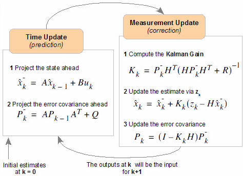 Figure: Stages
of the Kalman Filter
Figure: Stages
of the Kalman Filter
The
Kalman filter basically consists of two stages. In the first
stage a mathematical state model is used to make a prediction about the
system state. In the next stage this state prediction is
compared
to measured state values. The difference between the
predicted
and measured state is moderated based on estimated noise and error in
the system and measurements, and a state estimation is output.
The output estimation is then used in conjuction with the
mathematical state model to predict the future state during the next
time update, and the cycle begins again.
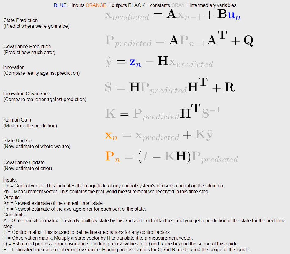 Figure: Kalman
Filter Equations
Figure: Kalman
Filter Equations
The figure above displays
the equations and variables that make up a basic Kalman filter.
The meaning of most of the variables is fairly obvious.
It
should be noted that the patameters Q and R represent the estimated
expected error in the system model and in the measurements.
By
changing these values, one can effectively "tune" the Kalman filter to
obtain better results. If, for example, the measurements of a
system are considered to be very accurate, a small value for R would be
used. In this situation the Kalman filter output would follow
the
measure values more closely than the predicted state estimate.
Linear Kalman Filter for
Positioning
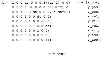 Figure: State
Transition and State Model Matrices
Figure: State
Transition and State Model Matrices for Positioning
Extended Kalman Filter
(Quaternions)
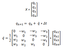 Figure: Kalman
State Model for Quaternions & Orientation
Figure: Kalman
State Model for Quaternions & Orientation
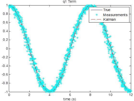
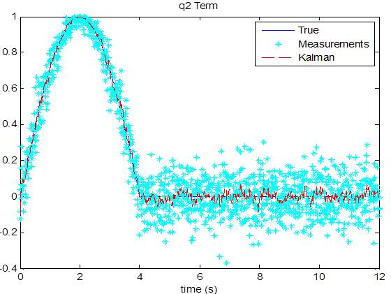
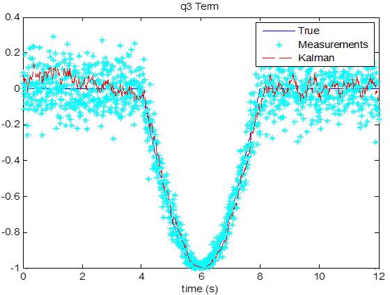
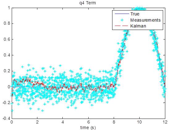
As can be seen in the plots
above, the
Kalman filter is providing a better estimate of the system quaternion
that defines orientation. These results will be furthur
improved
once proper values for Q and R have been determined. The team
is
currently in the process of finding these values, which involves
tracking and combining sensor error values as the quaternions are
calculated.
Even though the proper values of Q and R have yet to
be determined, the estimated quaternion is still much improved over the
measured values. The videos below show the visualization of
the
sensor with measurement values and with filtered quaternion values.